
So far in our discussion of recurrent neural networks, you have learned:
- The basic intuition behind recurrent neural networks
- The vanishing gradient problem that historically impeded the progress of recurrent neural networks
- How long short-term memory networks (LSTMs) help to solve the vanishing gradient problem
It's now time to build your first recurrent neural network! More specifically, this tutorial will teach you how to build and train an LSTM to predict the stock price of Facebook (FB).
Table of Contents
You can skip to a specific section of this Python recurrent neural network tutorial using the table of contents below:
- Downloading the Data Set For This Tutorial
- Importing The Libraries You'll Need For This Tutorial
- Importing Our Training Set Into The Python Script
- Applying Feature Scaling To Our Data Set
- Specifying The Number Of Timesteps For Our Recurrent Neural Network
- Finalizing Our Data Sets By Transforming Them Into NumPy Arrays
- Importing Our TensorFlow Libraries
- Building Our Recurrent Neural Network
- Adding Our First LSTM Layer
- Adding Some Dropout Regularization
- Adding Three More LSTM Layers With Dropout Regularization
- Adding The Output Layer To Our Recurrent Neural Network
- Compiling Our Recurrent Neural Network
- Fitting The Recurrent Neural Network On The Training Set
- The Full Code For This Tutorial
- Final Thoughts
Downloading the Data Set For This Tutorial
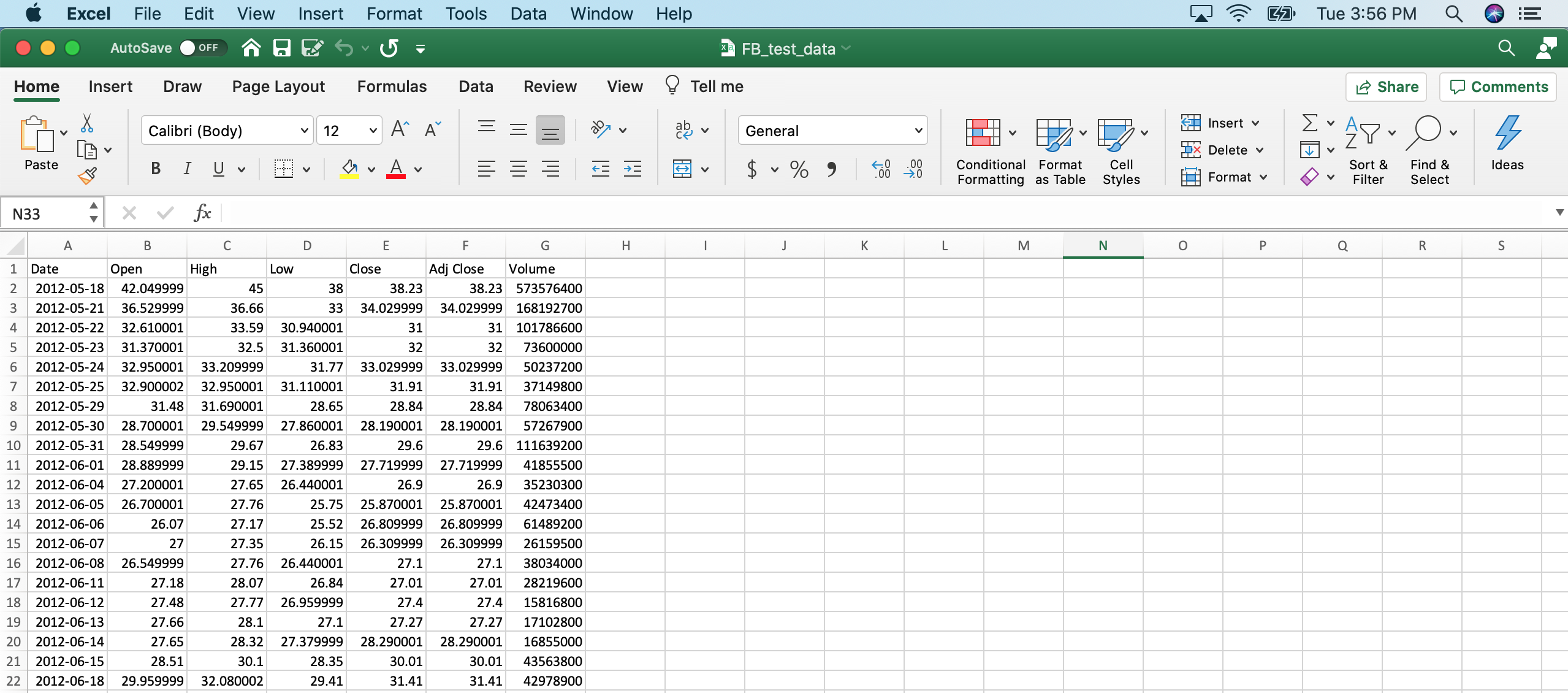
To proceed through this tutorial, you will need two download two data sets:
- A set of training data that contains information on Facebook's stock price from teh start of 2015 to the end of 2019
- A set of test data that contains information on Facebook's stock price during the first month of 2020
Our recurrent neural network will be trained on the 2015-2019 data and will be used to predict the data from January 2020.
You can download the training data and test data using the links below:
Each of these data sets are simply exports from Yahoo! Finance. They look like this (when opened in Microsoft Excel):
Once the files are downloaded, move them to the directory you'd like to work in and open a Jupyter Notebook.
Importing The Libraries You'll Need For This Tutorial
This tutorial will depend on a number of open-source Python libraries, including NumPy, pandas, and matplotlib.
Let's start our Python script by importing some of these libraries:
import numpy as np

import pandas as pd

import matplotlib.pyplot as plt
Importing Our Training Set Into The Python Script
The next task that needs to be completed is to import our data set into the Python script.
We will initially import the data set as a pandas DataFrame using the read_csv method. However, since the keras module of TensorFlow only accepts NumPy arrays as parameters, the data structure will need to be transformed post-import.
Let's start by importing the entire .csv file as a DataFrame:
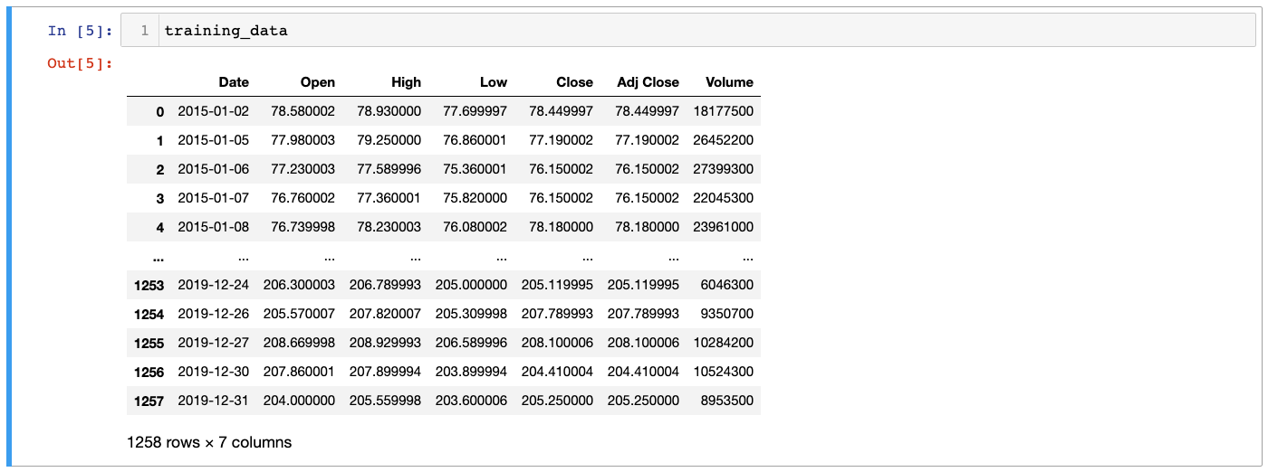
training_data = pd.read_csv('FB_training_data.csv')You will notice in looking at the DataFrame that it contains numerous different ways of measuring Facebook's stock price, including opening price, closing price, high and low prices, and volume information:
We will need to select a specific type of stock price before proceeding. Let's use Close, which indicates the unadjusted closing price of Facebook's stock.
Now we need to select that column of the DataFrame and store it in a NumPy array. Here is the command to do this:
training_data = training_data.iloc[:, 1].valuesNote that this command overwrites the existing training_data variable that we had created previously.
You can now verify that our training_data variable is indeed a NumPy array by running type(training_data), which should return:
numpy.ndarrayApplying Feature Scaling To Our Data Set
Let's now take some time to apply some feature scaling to our data set.
As a quick refresher, there are two main ways that you can apply featuer scaling to your data set:
- Standardization
- Normalization
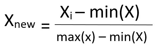
We'll be using normalization to build our recurrent neural network, which involves subtracting the minimum value of the data set and then dividing by the range of the data set.
Here is the normalization function defined mathematically:
Fortunately, scikit-learn makes it very easy to apply normalization to a dataset using its MinMaxScaler class.
Let's start by importing this class into our Python script. The MinMaxScaler class lives within the preprocessing module of scikit-learn, so the command to import the class is:
from sklearn.preprocessing import MinMaxScalerNext we need to create an instance of this class. We will assign the newly-created object to a variable called scaler. We will be using the default parameters for this class, so we do not need to pass anything in:
scaler = MinMaxScaler()Since we haven't specified any non-default parameters, this will scale our data set so that every observation is between 0 and 1.
We have created our scaler object but our training_data data set has not yet been scaled. We need to use the fit_transform method to modify the original data set. Here's the statement to do this:
training_data = scaler.fit_transform(training_data.reshape(-1, 1))Specifying The Number Of Timesteps For Our Recurrent Neural Network
The next thing we need to do is to specify our number of timesteps. Timesteps specify how many previous observations should be considered when the recurrent neural network makes a prediction about the current observation.
We will use 40 timesteps in this tutorial. This means that for every day that the neural network predicts, it will consider the previous 40 days of stock prices to determine its output. Note that since there are only ~20 trading days in a given month, using 40 timesteps means we're relying on stock price data from the previous 2 months.
So how do we actually specify the number of timesteps within our Python script?
It's done through creating two special data structures:
- One data structure that we'll call
x_training_datathat contains the last 40 stock price observations in the data set. This is the data that the recurrent neural network will use to make predictions. - One data structure that we'll call
y_training_datathat contains the stock price for the next trading day. This is the data point that the recurrent neural network is trying to predict.
To start, let's initialize each of these data structures as an empty Python list:
x_training_data = []

y_training_data =[]
Now we will use a for loop to populate the actual data into each of these Python lists. Here's the code (with further explanation of the code after the code block):
for i in range(40, len(training_data)):

    x_training_data.append(training_data[i-40:i, 0])

    y_training_data.append(training_data[i, 0])
Let's unpack the components of this code block:
- The
range(40, len(training_data))function causes the for loop to iterate from40to the last index of the training data. - The
x_training_data.append(training_data[i-40:i, 0])line causes the loop to append the 40 preceding stock prices tox_training_datawith each iteration of the loop. - Similarly, the
y_training_data.append(training_data[i, 0])causes the loop to append the next day's stock price toy_training_datawith each iteration of the loop.
Finalizing Our Data Sets By Transforming Them Into NumPy Arrays
TensorFlow is designed to work primarily with NumPy arrays. Because of this, the last thing we need to do is transform the two Python lists we just created into NumPy arrays.
Fortunately, this is simple. You simply need to wrap the Python lists in the np.array function. Here's the code:
x_training_data = np.array(x_training_data)

y_training_data = np.array(y_training_data)
One important way that you can make sure your script is running as intended is to verify the shape of both NumPy arrays.
The x_training_data array should be a two-directional NumPy array with one dimension being 40 (the number of timesteps) and the second dimension being len(training_data) - 40, which evaluates to 1218 in our case.
Similarly, the y_training_data object should be a one-dimensional NumPy array of length 1218 (which, again, is len(training_data) - 40).
You can verify the shape of the arrays by printing their shape attribute, like this:
print(x_training_data.shape)

print(y_training_data.shape)
This prints:
(1218, 40)

(1218,)
Both arrays have the dimensions you'd expect. However, we need to reshape our x_training_data object one more time before proceeding to build our recurrent neural network.
The reason for this is that the recurrent neural network layer available in TensorFlow only accepts data in a very specific format. You can read the TensorFlow documentation on this topic here.
To reshape the x_training_data object, I will use the np.reshape method. Here's the code to do this:
x_training_data = np.reshape(x_training_data, (x_training_data.shape[0],

                                               x_training_data.shape[1],

                                               1))
Now let's print the shape of x_training_data once again:
print(x_training_data.shape)This outputs:
(1218, 40, 1)Our arrays have the desired shape, so we can proceed to building our recurrent neural network.
Importing Our TensorFlow Libraries
Before we can begin building our recurrent neural network, we'll need to import a number of classes from TensorFlow. Here are the statements you should run before proceeding:
from tensorflow.keras.models import Sequential

from tensorflow.keras.layers import Dense

from tensorflow.keras.layers import LSTM

from tensorflow.keras.layers import Dropout
Building Our Recurrent Neural Network
It's now time to build our recurrent neural network.
The first thing that needs to be done is initializing an object from TensorFlow's Sequential class. As its name implies, the Sequential class is designed to build neural networks by adding sequences of layers over time.
Here's the code to initialize our recurrent neural network:
rnn = Sequential()As with our artificial neural networks and convolutional neural networks, we can add more layers to this recurrent neural network using the add method.
Adding Our First LSTM Layer
The first layer that we will add is an LSTM layer. To do this, pass an invocation of the LSTM class (that we just imported) into the add method.
The LSTM class accepts several parameters. More precisely, we will specify three arguments:
- The number of LSTM neurons that you'd like to include in this layer. Increasing the number of neurons is one method for increasing the dimensionality of your recurrent neural network. In our case, we will specify
units = 45. return_sequences = True- this must always be specified if you plan on including another LSTM layer after the one you're adding. You should specifyreturn_sequences = Falsefor the last LSTM layer in your recurrent neural network.input_shape: the number of timesteps and the number of predictors in our training data. In our case, we are using40timesteps and only1predictor (stock price), so we will add
Here is the full add method:
rnn.add(LSTM(units = 45, return_sequences = True, input_shape = (x_training_data.shape[1], 1)))Note that I used x_training_data.shape[1] instead of the hardcoded value in case we decide to train the recurrent neural network on a larger model at a later date.
Adding Some Dropout Regularization
Dropout regularization is a technique used to avoid overfitting when training neural networks.
It involves randomly excluding - or "dropping out" - certain layer outputs during the training stage.
TensorFlow makes it easy to implement dropout regularization using the Dropout class that we imported earlier in our Python script. The Dropout class accepts a single parameter: the dropout rate.
The dropout rate indicates how many neurons should be dropped in a specific layer of the neural network. It is common to use a dropout rate of 20%. We will follow this convention in our recurrent neural network.
Here's how you can instruct TensorFlow to drop 20% of the LSTM layer's neuron during each iteration of the training stage:
rnn.add(Dropout(0.2))Adding Three More LSTM Layers With Dropout Regularization
We will now add three more LSTM layers (with dropout regularization) to our recurrent neural network. You will see that after specifying the first LSTM layer, adding more is trivial.
To add more layers, all that needs to be done is copying the first two add methods with one small change. Namely, we should remove the input_shape argument from the LSTM class.
We will keep the number of neurons (or units) and the dropout rate the same in each of the LSTM class invocations. Since the third LSTM layer we're adding in this section will be our last LSTM layer, we can remove the return_sequences = True parameter as mentioned earlier. Removing the parameter sets return_sequences to its default value of False.
Here's the full code to add our next three LSTM layers:
rnn.add(LSTM(units = 45, return_sequences = True))

rnn.add(Dropout(0.2))

rnn.add(LSTM(units = 45, return_sequences = True))

rnn.add(Dropout(0.2))

rnn.add(LSTM(units = 45))

rnn.add(Dropout(0.2))
This code is very repetitive and violates the DRY (Don't repeat yourself) principle of software development. Let's nest it in a loop instead:
for i in [True, True, False]:

    rnn.add(LSTM(units = 45, return_sequences = i))

    rnn.add(Dropout(0.2))
Adding The Output Layer To Our Recurrent Neural Network
Let's finish architecting our recurrent neural network by adding our output layer.
The output layer will be an instance of the Dense class, which is the same class we used to create the full connection layer of our convolutional neural network earlier in this course.
The only parameter we need to specify is units, which is the desired number of dimensions that the output layer should generate. Since we want to output the next day's stock price (a single value), we'll specify units = 1.
Here's the code to create our output layer:
rnn.add(Dense(units = 1))Compiling Our Recurrent Neural Network
As you'll recall from the tutorials on artificial neural networks and convolutional neural networks, the compilation step of building a neural network is where we specify the neural net's optimizer and loss function.
TensorFlow allows us to compile a neural network using the aptly-named compile method. It accepts two arguments: optimizer and loss. Let's start by creating an empty compile function:
rnn.compile(optimizer = '', loss = '')We now need to specify the optimizer and loss parameters.
Let's start by discussing the optimizer parameter. Recurrent neural networks typically use the RMSProp optimizer in their compilation stage. With that said, we will use the Adam optimizer (as before). The Adam optimizer is a workhorse optimizer that is useful in a wide variety of neural network architectures.
The loss parameter is fairly simple. Since we're predicting a continuous variable, we can use mean squared error - just like you would when measuring the performance of a linear regression machine learning model. This means we can specify loss = mean_squared_error.
Here's the final compile method:
rnn.compile(optimizer = 'adam', loss = 'mean_squared_error')Fitting The Recurrent Neural Network On The Training Set
It's now time to train our recurrent network on our training data.
To do this, we use the fit method. The fit method accepts four arguments in this case:
- The training data: in our case, this will be
x_training_dataandy_training_data - Epochs: the number of iterations you'd like the recurrent neural network to be trained on. We will specify
epochs = 100in this case. - The batch size: the size of batches that the network will be trained in through each epoch.
Here is the code to train this recurrent neural network according to our specifications:
rnn.fit(x_training_data, y_training_data, epochs = 100, batch_size = 32)Your Jupyter Notebook will now generate a number of printed outputs for every epoch in the training algorithm. They look like this:
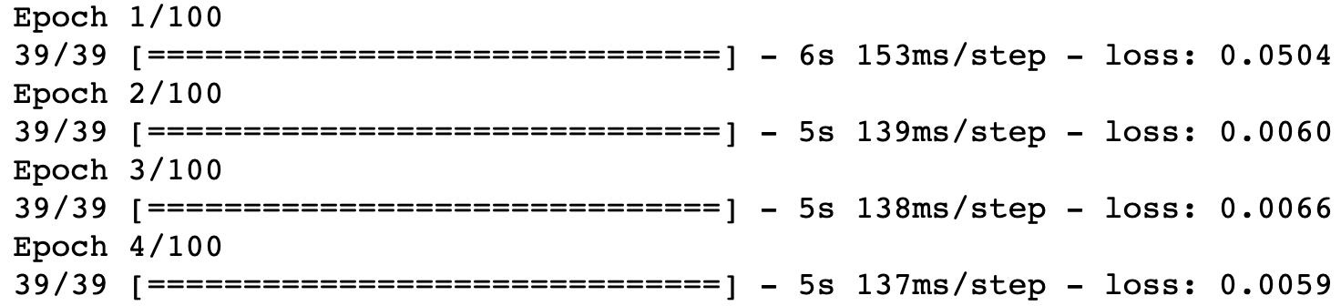
As you can see, every output shows how long the epoch took to compute as well as the computed loss function at that epoch.
You should see the loss function's value slowly decline as the recurrent neural network is fitted to the training data over time. In my case, the loss function's value declined from 0.0504 in the first iteration to 0.0017 in the last iteration.
Making Predictions With Our Recurrent Neural Network
We have built our recurrent neural network and trained it on data of Facebook's stock price over the last 5 years. It's now time to make some predictions!
Importing Our Test Data
To start, let's import the actual stock price data for the first month of 2020. This will give us something to compare our predicted values to.
Here's the code to do this. Note that it is very similar to the code that we used to import our training data at the start of our Python script:
test_data = pd.read_csv('FB_test_data.csv')

test_data = test_data.iloc[:, 1].values
If you run the statement print(test_data.shape), it will return (21,). This shows that our test data is a one-dimensional NumPy array with 21 entries - which means there were 21 stock market trading days in January 2020.
You can also generate a quick plot of the data using plt.plot(test_data). This should generate the following Python visualization:
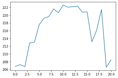
With any luck, our predicted values should follow the same distribution.
Building The Test Data Set We Need To Make Predictions
Before we can actually make predictions for Facebook's stock price in January 2020, we first need to make some changes to our data set.
The reason for this is that to predict each of the 21 observations in January, we will need the 40 previous trading days. Some of these trading days will come from the test set while the remainder will come from the training set. Because of this, some concatenation is necessary.
Unfortunately, you can just concatenate the NumPy arrays immediately. This is because we've already applied feature scaling to the training data but haven't applied any feature scaling to the test data.
To fix this, we need to re-import the original x_training_data object under a new variable name called unscaled_x_training_data. For consistency, we will also re-import the test data as a DataFrame called unscaled_test_data:
unscaled_training_data = pd.read_csv('FB_training_data.csv')

unscaled_test_data = pd.read_csv('FB_test_data.csv')
Now we can concatenate together the Open column from each DataFrame with the following statement:
all_data = pd.concat((unscaled_x_training_data['Open'], unscaled_test_data['Open']), axis = 0)This all_data object is a pandas Series of length 1279.
Now we need to create an array of all the stock prices from January 2020 and the 40 trading days prior to January. We will call this object x_test_data since it contains the x values that we'll use to make stock price predictions for January 2020.
The first thing you need to do is find the index of the first trading day in January within our all_data object. The statement len(all_data) - len(test_data) identifies this index for us.
This represents the upper bound of the first item in the array. To get the lower bound, just subtract 40 from this number. Said differently, the lower bound is len(all_data) - len(test_data) - 40.
The upper bound of the entire x_test_data array will be the last item in the data set. Accordingly, we can create this NumPy array with the following statement:
x_test_data = all_data[len(all_data) - len(test_data) - 40:].valuesYou can check whether or not this object has been created as desired by printing len(x_test_data), which has a value of 61. This makes sense - it should contain the 21 values for January 2020 as well as the 40 values prior.
The last step of this section is to quickly reshape our NumPy array to make it suitable for the predict method:
x_test_data = np.reshape(x_test_data, (-1, 1))Note that if you neglected to do this step, TensorFlow would print a handy message that would explain exactly how you'd need to transform your data.
Scaling Our Test Data
Our recurrent neural network was trained on scaled data. Because of this, we need to scale our x_test_data variable before we can use the model to make predictions.
x_test_data = scaler.transform(x_test_data)Note that we used the transform method here instead of the fit_transform method (like before). This is because we want to transform the test data according to the fit generated from the entire training data set.
This means that the transformation that is applied to the test data will be the same as the one applied to the training data - which is necessary for our recurrent neural network to make accurate predictions.
Grouping Our Test Data
The last thing we need to do is group our test data into 21 arrays of size 40. Said differently, we'll now create an array where each entry corresponds to a date in January and contains the stock prices of the 40 previous trading days.
The code to do this is similar to something we used earlier:
final_x_test_data = []

for i in range(40, len(x_test_data)):

    final_x_test_data.append(x_test_data[i-40:i, 0])

final_x_test_data = np.array(final_x_test_data)
Lastly, we need to reshape the final_x_test_data variable to meet TensorFlow standards.
We saw this previously, so the code should need no explanation:
final_x_test_data = np.reshape(final_x_test_data, (final_x_test_data.shape[0],

                                               final_x_test_data.shape[1],

                                               1))
Actually Making Predictions
After an absurd amount of data reprocessing, we are now ready to make predictions using our test data!
This step is simple. Simply pass in our final_x_test_data object into the predict method called on the rnn object. As an example, here is how you could generate these predictions and store them in an aptly-named variable called predictions:
predictions = rnn.predict(final_x_test_data)Let's plot these predictions by running plt.plot(predictions) (note that you'll need to run plt.clf() to clear your canvas first):
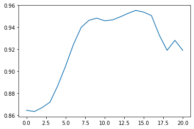
As you can see, the predicted values in this plot are all between 0 and 1. This is because our data set is still scaled! We need to un-scale it for the predictions to have any practical meaning.
The MinMaxScaler class that we used to originally scale our data set comes with a useful inverse_transform method to un-scale the data. Here's how you could un-scale the data and generate a new plot:
unscaled_predictions = scaler.inverse_transform(predictions)

plt.clf() #This clears the first prediction plot from our canvas

plt.plot(unscaled_predictions)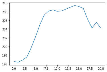
This looks much better! Anyone who's followed Facebook's stock price for any length of time can see that this seems fairly close to where Facebook has actually traded.
Let's generate plot that compares our predicted stock prices with Facebook's actual stock price:
plt.plot(unscaled_predictions, color = '#135485', label = "Predictions")

plt.plot(test_data, color = 'black', label = "Real Data")

plt.title('Facebook Stock Price Predictions')
The Full Code For This Tutorial
You can view the full code for this tutorial in this GitHub repository. It is also pasted below for your reference:
#Import the necessary data science libraries

import numpy as np

import pandas as pd

import matplotlib.pyplot as plt

#Import the data set as a pandas DataFrame

training_data = pd.read_csv('FB_training_data.csv')

#Transform the data set into a NumPy array

training_data = training_data.iloc[:, 1].values

#Apply feature scaling to the data set

from sklearn.preprocessing import MinMaxScaler

scaler = MinMaxScaler()

training_data = scaler.fit_transform(training_data.reshape(-1, 1))

#Initialize our x_training_data and y_training_data variables

#as empty Python lists

x_training_data = []

y_training_data =[]

#Populate the Python lists using 40 timesteps

for i in range(40, len(training_data)):

    x_training_data.append(training_data[i-40:i, 0])

    y_training_data.append(training_data[i, 0])


#Transforming our lists into NumPy arrays

x_training_data = np.array(x_training_data)

y_training_data = np.array(y_training_data)

#Verifying the shape of the NumPy arrays

print(x_training_data.shape)

print(y_training_data.shape)

#Reshaping the NumPy array to meet TensorFlow standards

x_training_data = np.reshape(x_training_data, (x_training_data.shape[0],

                                               x_training_data.shape[1],

                                               1))

#Printing the new shape of x_training_data

print(x_training_data.shape)

#Importing our TensorFlow libraries

from tensorflow.keras.models import Sequential

from tensorflow.keras.layers import Dense

from tensorflow.keras.layers import LSTM

from tensorflow.keras.layers import Dropout

#Initializing our recurrent neural network

rnn = Sequential()

#Adding our first LSTM layer

rnn.add(LSTM(units = 45, return_sequences = True, input_shape = (x_training_data.shape[1], 1)))

#Perform some dropout regularization

rnn.add(Dropout(0.2))

#Adding three more LSTM layers with dropout regularization

for i in [True, True, False]:

    rnn.add(LSTM(units = 45, return_sequences = i))

    rnn.add(Dropout(0.2))

#(Original code for the three additional LSTM layers)

# rnn.add(LSTM(units = 45, return_sequences = True))

# rnn.add(Dropout(0.2))

# rnn.add(LSTM(units = 45, return_sequences = True))

# rnn.add(Dropout(0.2))

# rnn.add(LSTM(units = 45))

# rnn.add(Dropout(0.2))

#Adding our output layer

rnn.add(Dense(units = 1))

#Compiling the recurrent neural network

rnn.compile(optimizer = 'adam', loss = 'mean_squared_error')

#Training the recurrent neural network

rnn.fit(x_training_data, y_training_data, epochs = 100, batch_size = 32)

#Import the test data set and transform it into a NumPy array

test_data = pd.read_csv('FB_test_data.csv')

test_data = test_data.iloc[:, 1].values

#Make sure the test data's shape makes sense

print(test_data.shape)

#Plot the test data

plt.plot(test_data)

#Create unscaled training data and test data objects

unscaled_training_data = pd.read_csv('FB_training_data.csv')

unscaled_test_data = pd.read_csv('FB_test_data.csv')

#Concatenate the unscaled data

all_data = pd.concat((unscaled_x_training_data['Open'], unscaled_test_data['Open']), axis = 0)

#Create our x_test_data object, which has each January day + the 40 prior days

x_test_data = all_data[len(all_data) - len(test_data) - 40:].values

x_test_data = np.reshape(x_test_data, (-1, 1))

#Scale the test data

x_test_data = scaler.transform(x_test_data)

#Grouping our test data

final_x_test_data = []

for i in range(40, len(x_test_data)):

    final_x_test_data.append(x_test_data[i-40:i, 0])

final_x_test_data = np.array(final_x_test_data)

#Reshaping the NumPy array to meet TensorFlow standards

final_x_test_data = np.reshape(final_x_test_data, (final_x_test_data.shape[0],

                                               final_x_test_data.shape[1],

                                               1))

#Generating our predicted values

predictions = rnn.predict(final_x_test_data)

#Plotting our predicted values

plt.clf() #This clears the old plot from our canvas

plt.plot(predictions)

#Unscaling the predicted values and re-plotting the data

unscaled_predictions = scaler.inverse_transform(predictions)

plt.clf() #This clears the first prediction plot from our canvas

plt.plot(unscaled_predictions)

#Plotting the predicted values against Facebook's actual stock price

plt.plot(unscaled_predictions, color = '#135485', label = "Predictions")

plt.plot(test_data, color = 'black', label = "Real Data")

plt.title('Facebook Stock Price Predictions')
Final Thoughts
In this tutorial, you learned how to build and train a recurrent neural network.
Here is a brief summary of what you learned:
- How to apply feature scaling to a data set that a recurrent neural network will be trained on
- The role of
timestepsin training a recurrent neural network - That TensorFlow primarily uses NumPy arrays as the data structure to train models with
- How to add
LSTMandDropoutlayers to a recurrent neural network - Why dropout regularization is commonly used to avoid overfitting when training neural networks
- That the
Denselayer from TensorFlow is commonly used as the output layer of a recurrent neural network - That the
compilationstep of building a neural network involves specifying its optimizer and its loss function - How to make predictions using a recurrent neural network
- That predictions make using a neural network trained on scaled data must be unscaled to be interpretable by humans